- ▶
- Heaters/Source
- ▶
- Agilent Heaters and SensorsMass Spectrometry, Scientific Supplies & ManufacturingScientific Instrument Services 5973 Source Heater Tamper Resistant Allen Wrench 5973/5975 Quad Sensor 5985 Source Heater Assembly Agilent Interface Heater Assembly 5971 Interface Heater
- ▶
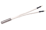
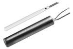
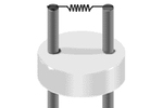
- Filaments
- LiteratureApplication Notes Adsorbent Resins Guide Mass Spec Tips SDS Sheets FAQ MS Calibration Compound Spectra Manuals MS Links/Labs/ Organizations MS Online Tools Flyers on Products/Services Scientific Supplies Catalog About Us NextAdvance Bullet Blender® Homogenizer Protocols Micro-Mesh® Literature Instrumentation Literature Agilent GC/MS Literature SIS News / E-Mail Newsletter NIST MS Database - Update Notifications

- ▶
- Application NotesNote 103: EPA Method 325B, Novel Thermal Desorption Instrument Modification to Improve Sensitivity Note 102: Identification of Contaminants in Powdered Beverages by Direct Extraction Thermal Desorption GC/MS Note 101: Identification of Contaminants in Powdered Foods by Direct Extraction Thermal Desorption GC/MS Note 100: Volatile and Semi-Volatile Profile Comparison of Whole Versus Cracked Versus Dry Homogenized Barley Grains by Direct Thermal Extraction Note 99: Volatile and Semi-Volatile Profile Comparison of Whole vs. Dry Homogenized Wheat, Rye and Barley Grains by Direct Thermal Extraction GC/MS Note 98: Flavor and Aroma Profiles of Truffle Oils by Thermal Desorption GC/MS Note 97: Flavor Profiles of Imported and Domestic Beers by Purge & Trap Thermal Desorption GC/MS Note 96: Reducing Warping in Mass Spectrometer Filaments, with SISAlloy® Yttria/Rhenium Filaments Note 95: Detection of Explosives on Clothing Material by Direct and AirSampling Thermal Desorption GC/MS Note 94: Detection of Nepetalactone in the Nepeta Cataria Plant by Thermal Desorption GC/MS Note 93: Detection of Benzene in Carbonated Beverages with Purge & Trap Thermal Desorption GC/MS Note 92: Yttria Coated Mass Spectrometer Filaments Note 91: AutoProbe DEP Probe Tip Temperatures Note 90: An Automated MS Direct Probe for use in an Open Access Environment Note 89: Quantitation of Organics via a Mass Spectrometer Automated Direct Probe Note 88: Analysis of Silicone Contaminants on Electronic Components by Thermal Desorption GC-MS Note 87: Design and Development of an Automated Direct Probe for a Mass Spectrometer Note 86: Simulation of a Unique Cylindrical Quadrupole Mass Analyzer Using SIMION 7.0. Note 85: Replacing an Electron Multiplier in the Agilent (HP) 5973 MSD Note 84: Vacuum Pump Exhaust Filters - Charcoal Exhaust Traps Note 83: Vacuum Pump Exhaust Filters - Oil Mist Eliminators Note 82: Vacuum Pump Exhaust Filters Note 81: Rapid Bacterial Chemotaxonomy By DirectProbe/MSD Note 80: Design, Development and Testing of a Microprocessor ControlledAutomated Short Path Thermal Desorption Apparatus Note 79: Volatile Organic Compounds From Electron Beam Cured and Partially Electron Beam Cured Packaging Using Automated Short Path Thermal Desorption Note 78: A New Solution to Eliminate MS Down-Time With No-Tool-Changing of Analytical GC Columns Note 77: The Determination of Volatile Organic Compounds in VacuumSystem Components Note 76: Determination of the Sensitivity of a CRIMS System Note 75: An Apparatus for Sampling Volatile Organics From LivePlant Material Using Short Path Thermal Desorption Note 74: Examination of Source Design in Electrospray-TOF Using SIMION 3D Note 73: The Analysis of Perfumes and their Effect on Indoor Air Pollution Note 72: 1998 Version of the NIST/EPA/NIH Mass Spectral Library, NIST98 Note 71: Flavor Profile Determination of Rice Samples Using Shor tPath Thermal Desorption GC Methods Note 70: Application of SIMION 6.0 To a Study of the Finkelstein Ion Source: Part II Note 69: Application of SIMION 6.0 To a Study of the Finkelstein Ion Source: Part 1 Note 68: Use of a PC Plug-In UV-Vis Spectrometer To Monitor the Plasma Conditions In GC-CRIMS Note 67: Using Chemical Reaction Interface Mass Spectrometry (CRIMS) To Monitor Bacterial Transport In In Situ Bioremediation Note 66: Probe Tip Design For the Optimization of Direct Insertion Probe Performance Note 65: Determination of Ethylene by Adsorbent Trapping and Thermal Desorption - Gas Chromatography Note 64: Comparison of Various GC/MS Techniques For the Analysis of Black Pepper (Piper Nigrum) Note 63: Determination of Volatile and Semi-Volatile Organics in Printer Toners Using Thermal Desorption GC Techniques Note 62: Analysis of Polymer Samples Using a Direct Insertion Probe and EI Ionization Note 61: Analysis of Sugars Via a New DEP Probe Tip For Use With theDirect Probe On the HP5973 MSD Note 60: Programmable Temperature Ramping of Samples Analyzed ViaDirect Thermal Extraction GC/MS Note 59: Computer Modeling of a TOF Reflectron With Gridless Reflector Using SIMION 3D Note 58: Direct Probe Analysis and Identification of Multicomponent Pharmaceutical Samples via Electron Impact MS Note 57: Aroma Profiles of Lavandula species Note 56: Mass Spec Maintenance & Cleaning Utilizing Micro-Mesh® Abrasive Sheets Note 55: Seasonal Variation in Flower Volatiles Note 54: Identification of Volatile Organic Compounds in Office Products Note 53: SIMION 3D v6.0 Ion Optics Simulation Software Note 52: Computer Modeling of Ion Optics in Time-of-Flight mass Spectrometry Using SIMION 3D Note 51: Development and Characterization of a New Chemical Reaction Interface for the Detection of Nonradioisotopically Labeled Analytes Using Mass Spectrometry (CRIMS) Note 50: The Analysis of Multiple Component Drug Samples Using a Direct Probe Interfaced to the HP 5973 MSD Note 49: Analysis of Cocaine Utilizing a New Direct Insertion Probe on a Hewlett Packard 5973 MSD Note 48: Demonstration of Sensitivity Levels For the Detection of Caffeine Using a New Direct Probe and Inlet for the HP 5973 MSD Note 47: The Application Of SIMION 6.0 To Problems In Time-of-Flight Mass Spectrometry Note 46: Delayed Extraction and Laser Desorption: Time-lag Focusing and Beyond Note 45: Application of SIMION 6.0 to Filament Design for Mass Spectrometer Ionization Sources Note 44: The Design Of a New Direct Probe Inlet For a Mass Spectrometer Note 43: Volatile Organic Composition In Blueberries Note 42: The Influence of Pump Oil Purity on Roughing Pumps Note 41: Hydrocarbon Production in Pine by Direct Thermal Extraction Note 40: Comparison of Septa by Direct Thermal Extraction Note 39: Comparison of Sensitivity Of Headspace GC, Purge and Trap Thermal Desorption and Direct Thermal Extraction Techniques For Volatile Organics Note 38: A New Micro Cryo-Trap For Trapping Of Volatiles At the Front Of a GC Capillary Column Note 37: Volatile Organic Emissions from Automobile Tires Note 36: Identification Of Volatile Organic Compounds In a New Automobile Note 35: Volatile Organics Composition of Cranberries Note 34: Selection Of Thermal Desorption and Cryo-Trap Parameters In the Analysis Of Teas Note 33: Changes in Volatile Organic Composition in Milk Over Time Note 32: Selection and Use of Adsorbent Resins for Purge and Trap Thermal Desorption Applications Note 31: Volatile Organic Composition in Several Cultivars of Peaches Note 30: Comparison Of Cooking Oils By Direct Thermal Extraction and Purge and Trap GC/MS Note 29: Analysis Of Volatile Organics In Oil Base Paints By Automated Headspace Sampling and GC Cryo-Focusing Note 28: Analysis Of Volatile Organics In Latex Paints By Automated Headspace Sampling and GC Cryo-Focusing Note 27: Analysis of Volatile Organics In Soils By Automated Headspace GC Note 26: Volatile Organics Present in Recycled Air Aboard a Commercial Airliner Note 25: Flavor and Aroma in Natural Bee Honey Note 24: Selection of GC Guard Columns For Use With the GC Cryo-Trap Note 23: Frangrance Qualities in Colognes Note 22: Comparison Of Volatile Compounds In Latex Paints Note 21: Detection and Identification Of Volatile and Semi-Volatile Organics In Synthetic Polymers Used In Food and Pharmaceutical Packaging Note 20: Using Direct Thermal Desorption to Assess the Potential Pool of Styrene and 4-Phenylcyclohexene In Latex-Backed Carpets Note 19: A New Programmable Cryo-Cooling/Heating Trap for the Cryo-Focusing of Volatiles and Semi-Volatiles at the Head of GC Capillary Columns Note 18: Determination of Volatile Organic Compounds In Mushrooms Note 17: Identification of Volatile Organics in Wines Over Time Note 16: Analysis of Indoor Air and Sources of Indoor Air Contamination by Thermal Desorption Note 14: Identification of Volatiles and Semi-Volatiles In Carbonated Colas Note 13: Identification and Quantification of Semi-Volatiles In Soil Using Direct Thermal Desorption Note 12: Identification of the Volatile and Semi-Volatile Organics In Chewing Gums By Direct Thermal Desorption Note 11: Flavor/Fragrance Profiles of Instant and Ground Coffees By Short Path Thermal Desorption Note 10: Quantification of Naphthalene In a Contaminated Pharmaceutical Product By Short Path Thermal Desorption Note 9: Methodologies For the Quantification Of Purge and Trap Thermal Desorption and Direct Thermal Desorption Analyses Note 8: Detection of Volatile Organic Compounds In Liquids Utilizing the Short Path Thermal Desorption System Note 7: Chemical Residue Analysis of Pharmaceuticals Using The Short Path Thermal Desorption System Note 6: Direct Thermal Analysis of Plastic Food Wraps Using the Short Path Thermal Desorption System Note 5: Direct Thermal Analysis Using the Short Path Thermal Desorption System Note 4: Direct Analysis of Spices and Coffee Note 3: Indoor Air Pollution Note 2: Detection of Arson Accelerants Using Dynamic Headspace with Tenax® Cartridges Thermal Desorption and Cryofocusing Note 1: Determination of Off-Odors and Other Volatile Organics In Food Packaging Films By Direct Thermal Analysis-GC-MS Tech No. "A" Note 14: Elimination of "Memory" Peaks in Thermal Desorption Improving Sensitivity in the H.P. 5971 MSD and Other Mass Spectrometers - Part I of II Improving Sensitivity in the H.P. 5971 MSD and Other Mass Spectrometers- Part II of II Adsorbent Resins Guide Development and Field Tests of an Automated Pyrolysis Insert for Gas Chromatography. Hydrocarbon Production in Pine by Direct Thermal Extraction A New Micro Cryo-Trap for the Trapping of Volatiles at the Front of a GC Capillary (019P) - Comparison of Septa by Direct Thermal Extraction Volatile Organic Composition in Blueberry Identification of Volatile Organic Compounds in Office Products Detection and Indentification of Volatiles in Oil Base Paintsby Headspace GC with On Column Cryo-Trapping Evaluation of Septa Using a Direct Thermal Extraction Technique INFLUENCE OF STORAGE ON BLUEBERRY VOLATILES Selection of Thermal Desorption and Cryo-Trap Parameters in the Analysis of Teas Redesign and Performance of a Diffusion Based Solvent Removal Interface for LC/MS The Design of a New Direct Probe Inlet for a Mass Spectrometer Analytes Using Mass Spectrometry (CRIMS) Application of SIMION 6.0 to Filament Design for Mass Spectrometer Ionization Sources A Student Guide for SIMION Modeling Software Application of SIMION 6.0 to Problems in Time-of-flight Mass Spectrometry Comparison of Sensitivity of Headspace GC, Purge and TrapThermal Desorption and Direct Thermal Extraction Techniques forVolatile Organics The Influence of Pump Oil Purity on Roughing Pumps Analysis of Motor Oils Using Thermal Desorption-Gas Chromatography-Mass Spectrometry IDENTIFICATION OF VOLATILE ORGANIC COMPOUNDS IN PAPER PRODUCTS Computer Modeling of Ion Optics in Time-of-Flight mass Spectrometry using SIMION 3D Seasonal Variation in Flower Volatiles Development of and Automated Microprocessor Controlled Gas chromatograph Fraction Collector / Olfactometer Delayed Extraction and Laser Desorption: Time-lag Focusing and Beyond A New Micro Cryo-Trap for the Trapping of Volatiles at the Front of a GC Column Design of a Microprocessor Controlled Short Path Thermal Desorption Autosampler Computer Modeling of Ion Optics in Time-of-Flight Mass Spectrometry Using SIMION 3D Thermal Desorption Instrumentation for Characterization of Odors and Flavors
- ▶
- Note 45: Application of SIMION 6.0 to Filament Design for Mass Spectrometer Ionization Sources (This Page)
By Steven Colby, Christopher W. Baker and John J. Manura
1999
INTRODUCTION
We investigate and analyze methods for improving the source geometry of a quadrupole mass spectrometer. As an example of the techniques employed, the effects of the orientation of a filament wire are explored. Emphasis is placed on the application of a software program, SIMION 3D, for the simulation of ion optics. In order for these results to be of general use, a generic ion source is modeled and the simulation process is described in sufficient detail so that the reader can use these methods on more specific examples.
Software
The results reported in this poster were generated with the ion optics program, SIMION 3D v.6.0. This software was developed by David Dahl at the Idaho National Engineering Laboratory1. The latest version allows for greatly expanded simulation capabilities. These include larger array sizes (10 million points) and three dimensional modeling. The new capabilities of dynamic parameter variation, time varying potentials, and user programming are also employed in the work below.
Fig. 1 - Simulated quadrupole Mass Spectrometer
Simulation
SIMION was used to model the quadrupole mass spectrometer shown in Figure 1. The simulation was divided into five sections. Each of these was designed and "refined" individually. (Refining is SIMION's method of calculating the potentials on non-electrode points.) The sections are then placed on an Ion Optics Bench (IOB) in their proper positions. The IOB feature allows items to be reused in different simulations. For example, parts of the quadrupole mass filter in this work were taken from an example that is included with the software. The IOB also permits the use of pieces whose symmetries differ. It is often helpful to incorporate elements of symmetry in the simulation, because they dramatically reduce the number of array points required. Likewise, sections of the simulation can have a different number of grid points per unit area. This allows for more accurate simulations where needed, as around the filament, without requiring such high precision everywhere else in the instrument.
The five sections (or instances) used in our experiments were a magnet, the source, the region between the source and the start of the quadrupoles, the quadrupoles, and the volume including the end of the quadrupoles and detector. The source instance consisted of a cylindrical piece (1.5 cm long X 1.0 cm dia.) with a flat plate at one end and a "repeller" on the side facing away from the quadrupoles. The plate included a 2 mm aperture to pass ions into the mass analyzer. Two planes of symmetry along the main axis of the instrument were used to divide the number of points in the calculation by a factor of four. A 2 x 3 mm slit was placed in the source to allow electrons from the filament to enter. (Because of the symmetry used, our simulation included two identical filaments and slits.) The filaments and slits were either oriented parallel or perpendicular to the principal axis of the instrument. The filament was placed 2 mm from the source cylinder. A magnetic instance was placed over the source, so that an appropriate magnetic field was generated between the two filaments. The instance between the source and the quadrupoles included an electrode with another 2 mm aperture. In many actual instruments, an einzel lens is placed in this area. The instance also incorporated a section of the quadrupoles in order to properly model the transition between these two regions of the instrument. The quadrupoles were modeled in two dimensions and then "extruded" along the axis of the instrument in the IOB. The final instance modeled the transition between the end of the quadrupoles and the detector.
Table 1. DC Potentials
Repeller +40.0V
Filament -70.0
Source cylinder 0.0
Lens after source 0.0
Quadrupole axis -8.0
Detector front -100.0
Detector Back -1500.0
Electrons and ions were simulated using SIMION's trajectory calculations. The DC potentials used are shown in Table 1. The potentials of the quadrupoles were varied at a radio frequency of 1.1 MHz in order to pass ions of 100 m/z. Control of the time dependent potentials was accomplished using SIMION's user programming interface. Each simulation was performed using groups of ions. Within each group electrons were assumed to leave a filament at 10 different points covering a linear range of 2 mm. At each of these points five electrons were generated with different angular trajectories. All electrons were given 0.25 eV of kinetic energy. Before the simulation of each group, a random number was generated for use in determining where electrons should turn into positive ions of 100 m/z. This was intended to simulate the electron impact ionization of neutral species. The simulation was repeated a large number of times in order to model the random generation of ions in the region between the two filaments.
Fig. 2 - Example Code Fragment For Simulated Ionization. (click here for full code, 4K)
 seg Other_Actions
 ;
 rcl ionized ; check to see
if we have already ionized
 x>0 exit ; if yes, don't
do it twice
 rcl Ion_Px_gu ; Get ion position
 rcl IonStart - ; subtract
the starting position
 abs ; take absolute value
 rcl Ionplace ; recall ionization
place
 x>y exit ; if we aren't there
yet we leave
 ;
 mark ; otherwise: record
position
 ;
 rcl IonColor ; recall new
color
 sto Ion_Color ; change the
ions color
 ;
 rcl IonCharge ; recall new
charge
 sto Ion_Charge ; change the
ions charge
 ;
 rcl IonMass ; recall new
mass
 sto Ion_Mass ; change the
ions mass
 ;
 rand 2 * 1 - ; random # between
1 and -1
 rcl PercentEnergyVar * ;
multiply by the energy variation
 rcl IonEnergy * ; multiply
by the average energy
 rcl IonEnergy + ; add to
the average energy
 ; to get new energy
 rcl ion_mass ; recall ion
mass
 x><y ; swap x and y
 >spd ; convert to speed
 sto speed ; hold in temp
variable
 ; converted new energy to
speed
 360 rand * ; get a random
el angle
180 rand * ; get a random
az angle
 rcl speed ;
 ; now x= speed, y=az, z=el
 >r3d ; convert to rectangular
3d coordinates
 sto Ion_Vx_mm ; change the
ions velocity
 rlup
 sto Ion_Vy_mm
 rlup
 sto Ion_Vz_mm
 1 sto Ionized ; change boolean
(we have done it)
 exit ; done
The conversion of electrons to ions was handled using SIMION's user programming interface. An example of the code used is shown in Figure 2. This fragment illustrates the use of a previously calculated random distance (ionposit) to determine where ionization should occur. Commands are then executed to change the mass, charge, and display color of the particle. Further code then gives the new ion a new kinetic energy and direction. (Ions started with thermal energy +/- 10%.) The section of code shown is executed once every time SIMION calculates a step in the trajectory simulation. The programming language used is designed to compile directly to assembly code resulting in very fast calculations. The complete source code for all user programs used in this simulation is available on the internet2.
Fig. 3 - Sample Simulations (In A and B, Only the source region is shown. Views are along the y-axis).
 A
A
 B
B
 C
C
Results
Figure 3 shows the simulation of three ion groups. These are intended to show examples of the possible fates of the simulated ions. In the first case (A), ions are formed too close to the electron slit. They are, therefore, drawn back toward the filament. This was the most common path for ions to take. In the second case, ions are generated closer to the center of the source and, therefore, are eliminated by striking the front and side walls. In the final case, ions are formed very close to the center of the source region. Some of these ions reach the detector. However, the randomly directed initial thermal kinetic energy is sufficient to prevent most of these ions from reaching the detector.
Fig. 4 - Location Of ion Impacts For Parallel and Perpendicular
Filaments 
The probabilities of ion elimination occurring in each region of the instrument are summarized in Figure 4. This figure shows the results obtained when the filament was oriented parallel or perpendicular to the principal axis of the instrument. In either case, over 64% of the ions are lost through the filament opening. This is due to both the magnetic and electric fields of the source. The fraction of ions lost through this route is a function of the size and depth of the rectangular opening used to admit electrons into the source. A plot of potential energy contours of the source is shown in Figure 5. Ions are accelerated in directions perpendicular to the red lines shown. It is clear that only in the center region are ions directed towards the exit aperture. Those ions that do move towards the exit are accelerated into the plane of Figure 5 (xz plane) by the magnetic field. As a result, the ions that strike the front plate of the source do so on average below the level of the principal instrument axis. As was shown in Figure 4, those ions that do not travel towards the filament still have only a small chance of reaching the detector. The parallel orientation of the filament decreases the probability of ion detection by approximately 50%. This result was unexpected since a greater fraction of the electrons from the parallel filament pass close to the center axis of the instrument.
Fig. 5 - Potential energy Contours Of the Source Region
Fig. 6 - Screen Capture Showing the Ion Optics Bench and Parameter Variation Menu
Using SIMION's data recording menu, it is possible to determine the starting positions of the ions that reach the detector. This enables us to determine the zone in which detectable ions may be generated. The volumes found were approximately 0.15 x 1.7 x 1.4 mm for the perpendicular filament and 2.2 x 0.11 x 1.2 mm for the parallel filament orientation. This volume (~0.3 mm3) is quite small relative to the volume of the source.
Limitations Of the Simulation
Our goal in this presentation has been to demonstrate methods for instrument analysis and design rather than to characterize a specific instrument. However, as with any computer modeling, there are limitations to these simulations that must be kept in mind when analyzing the results. For example, the user program allows electrons to generate ions before they reach a significant kinetic energy. The system has also not been optimized so the potentials listed in Table 1 are not likely to be the best for ion collection in this system. Likewise, the specific geometry used was not based on an actual instrument or an optimal design. We have also not included the einzel lens found in many commercial instruments. This will certainly have a dramatic influence on the collection efficiency of ions.
Current Work
Our current work involves changes in the user program so that ions will only be generated in a volume slightly larger than the ion acceptance zone. This will dramatically improve the speed of simulations. We will then add an einzel lens before the quadrupoles and attempt to optimize instrument conditions. Optimization will be accomplished using SIMION's variable adjust utility. This option permits the user to change simulation parameters at any point during the trajectory calculations. A sample menu is shown in Figure 6. (This figure shows part of the IOB graphical user interface. Part of the instrument shown has been removed to reveal the interior.) In this example, variables, including percent tune, m/z, and lens potential, can be changed by typing in the appropriate values. The flight of ions is affected immediately.
Conclusions
We have demonstrated the use of SIMION 3D in modeling the source region of a quadrupole mass spectrometer. The software is an excellent tool for the investigation of ion optics within the instrument. We believe that the work of David Dahl will contribute to a large variety of applications.
References
1. David A. Dahl 43ed ASMS Conference on Mass Spectrometry and Allied Topics, May 21-26 1995, Atlanta, Georgia, pg 717.